Neal's Funnel • sbcrs

library(sbcrs)
library(rstan)
#> Loading required package: StanHeaders
#> Loading required package: ggplot2
#> rstan (Version 2.19.2, GitRev: 2e1f913d3ca3)
#> For execution on a local, multicore CPU with excess RAM we recommend calling
#> options(mc.cores = parallel::detectCores()).
#> To avoid recompilation of unchanged Stan programs, we recommend calling
#> rstan_options(auto_write = TRUE)

In this example, we will calibrate two versions of Neal’s funnel.¹

\[ p(y,x) = \mathsf{normal}(y|0,3) * \prod_{n=1}^9 \mathsf{normal}(x_n|0,\exp(y/2)) \]

When parameterized in terms of \(x_n\) and \(y\), this model is extremely difficult for Stan to sample from. Per the Stan User’s Guide: “The probability contours are shaped like ten-dimensional funnels. The funnel’s neck is particularly sharp because of the exponential function applied to \(y\).” Ideally, simulation-based calibration should detect the sampling pathologies in this model.

The stan code for this model (without re-parameterization) is:

parameters {
  real y;
  vector[9] x;
}
model {
  y ~ normal(0, 3);
  x ~ normal(0, exp(y/2));
}

Compile the Stan model:

funnel <- stan_model(file = system.file('stan', 'funnel.stan', package = 'sbcrs'))

Create an SBC object called sbc1 with functions to: 1) generate simulated values of x and y, and 2) call rstan::sampling, passing in funnel as the model to be sampled.

sbc1 <- SBC$new(
  params = function(seed, data) {
    set.seed(seed + 10)
    y <- rnorm(1, 0, 3)
    x <- rnorm(9, 0, exp(y/2))
    list(y = y, x = x)
  }, 
  sampling = function(seed, data, params, modeled_data, iters) {
    sampling(funnel, data = data, seed = seed, chains = 1, iter = 2 * iters, warmup = iters)
  })

Calibration involves generating data and parameters, and sampling from a Stan model many times. To speed up this process, take advantage of all of your machine’s cores.

doParallel::registerDoParallel(cores = parallel::detectCores())

Perform the calibration.

sbc1$calibrate(N = 256, L = 50)
sbc1$plot()

sbc1$plot('y')

sbc1$plot('x')

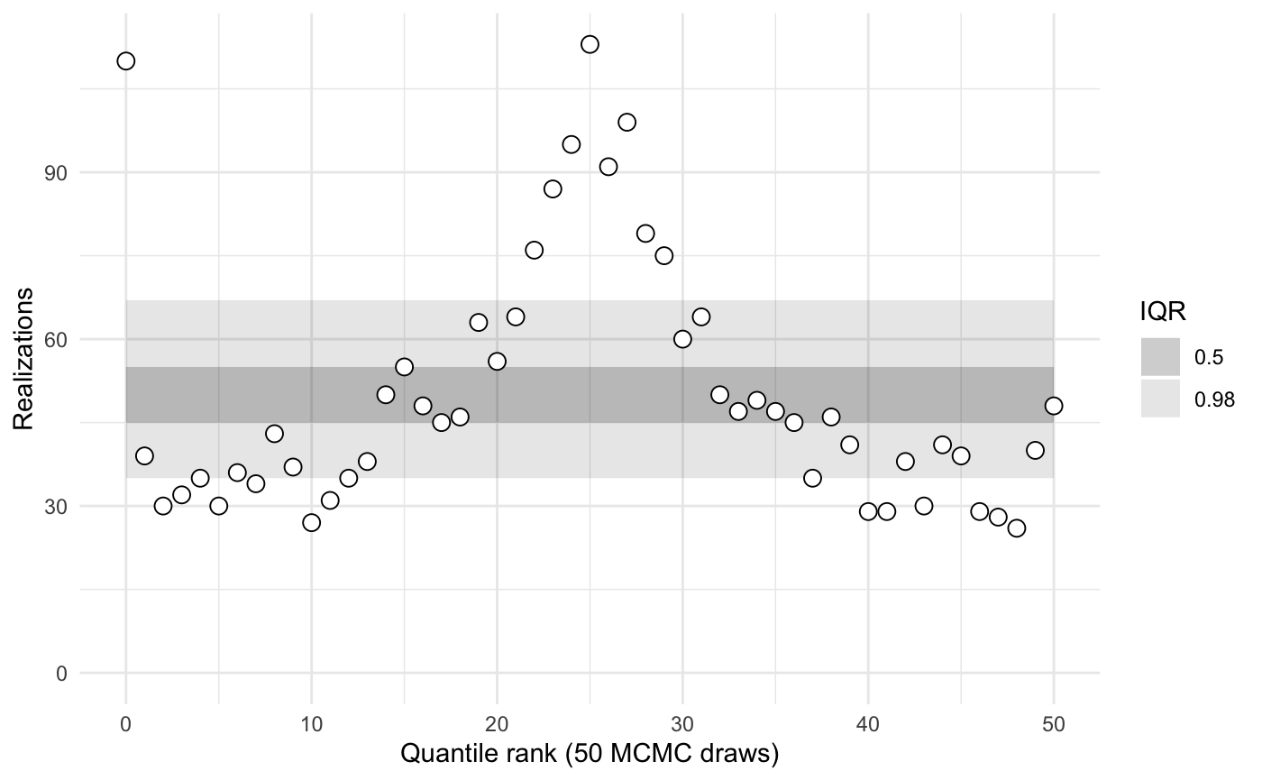
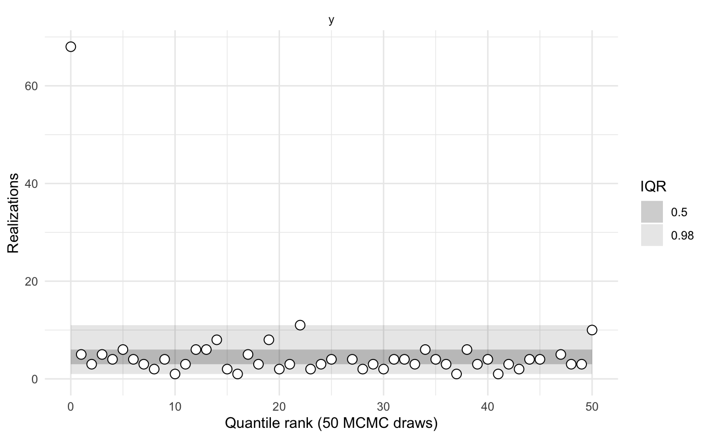
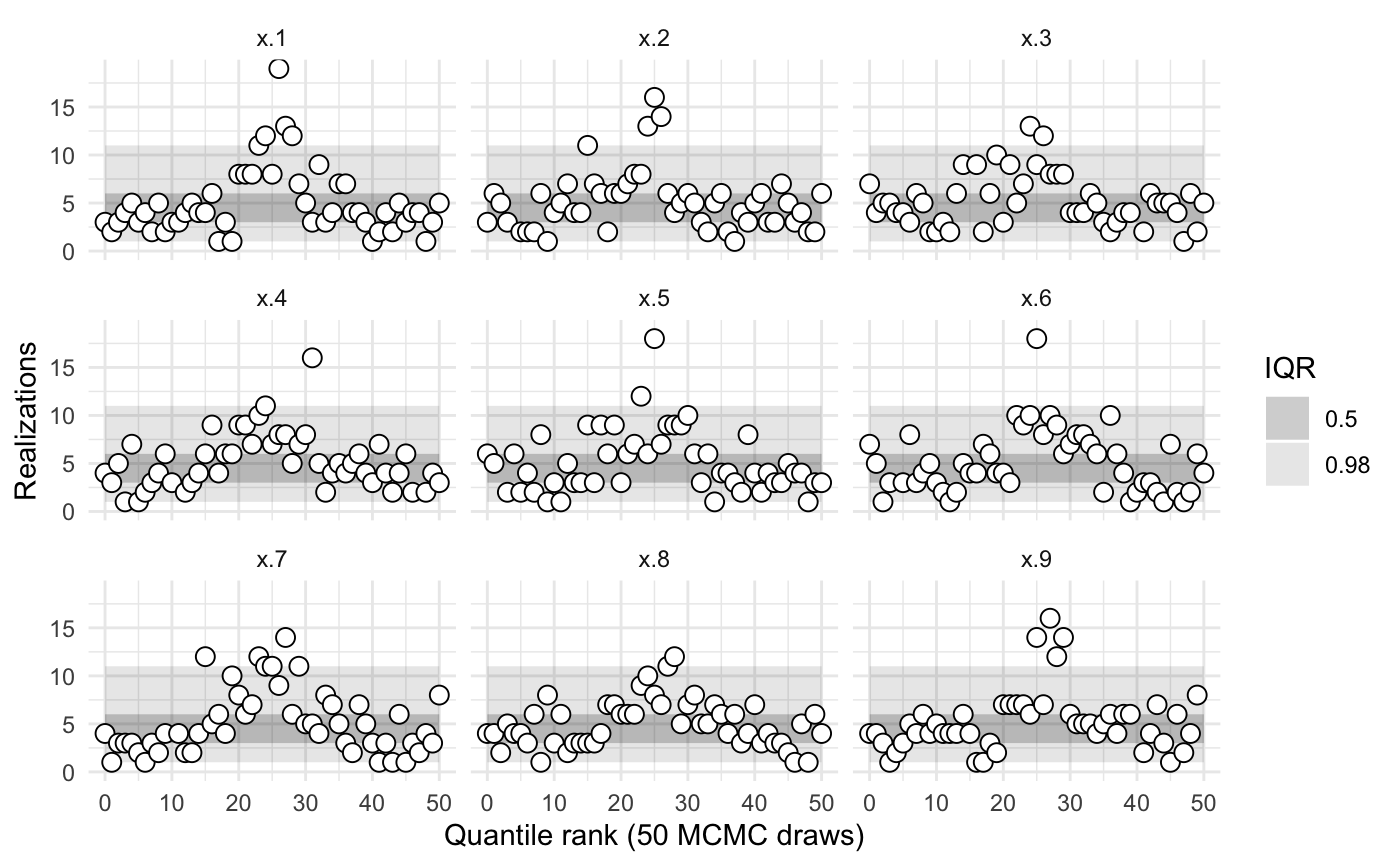
sbc1$summary()
#> 
#> 
#>    iq expected.outside actual.outside
#>  0.50             0.50      0.7647059
#>  0.98             0.02      0.4117647

The model is evidently poorly conditioned.

The reparameterized model is based on new primitives: x_raw and y_raw, which follow independent, standard normal distributions. From these newly defined primitives, it then builds up x and y based on their analytical definitions (see above). The stan code for the reparameterized model is:

parameters {
  real y_raw;
  vector[9] x_raw;
}
transformed parameters {
  real y;
  vector[9] x;

  y = 3.0 * y_raw;
  x = exp(y/2) * x_raw;
}
model {
  y_raw ~ std_normal(); // implies y ~ normal(0, 3)
  x_raw ~ std_normal(); // implies x ~ normal(0, exp(y/2))
}

Compile the (reparameterized) Stan model:

funnel_reparameterized <- stan_model(file = system.file('stan', 'funnel_reparameterized.stan', package = 'sbcrs'))

Create an SBC object called sbc2a with functions to: 1) generate simulated values of x_raw and y_raw, and 2) call rstan::sampling, passing in funnel_reparameterized as the model to be sampled.

sbc2a <- SBC$new(
  params = function(seed, data) {
    set.seed(seed + 10)
    y_raw <- rnorm(1, 0, 1)
    x_raw <- rnorm(9, 0, 1)
    list(y_raw = y_raw, x_raw = x_raw)
  }, 
  sampling = function(seed, data, params, modeled_data, iters) {
    sampling(funnel_reparameterized, data = data, seed = seed, chains = 1, iter = 2 * iters, warmup = iters)
  })

Perform the calibration.

sbc2a$calibrate(N = 256, L = 50)
sbc2a$plot()

sbc2a$plot('y_raw')

sbc2a$plot('x_raw')

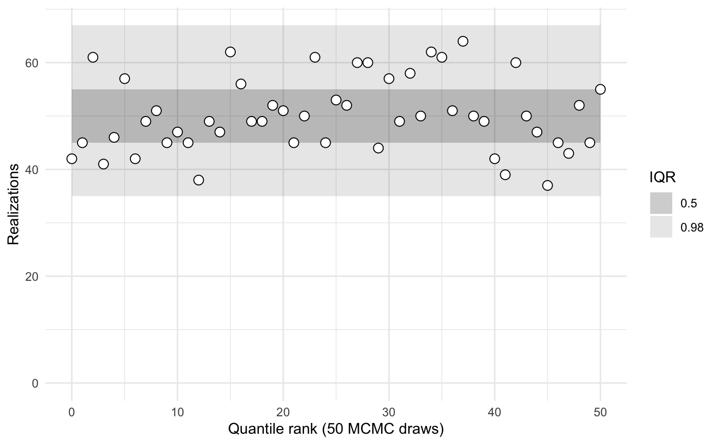
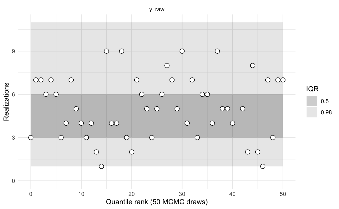
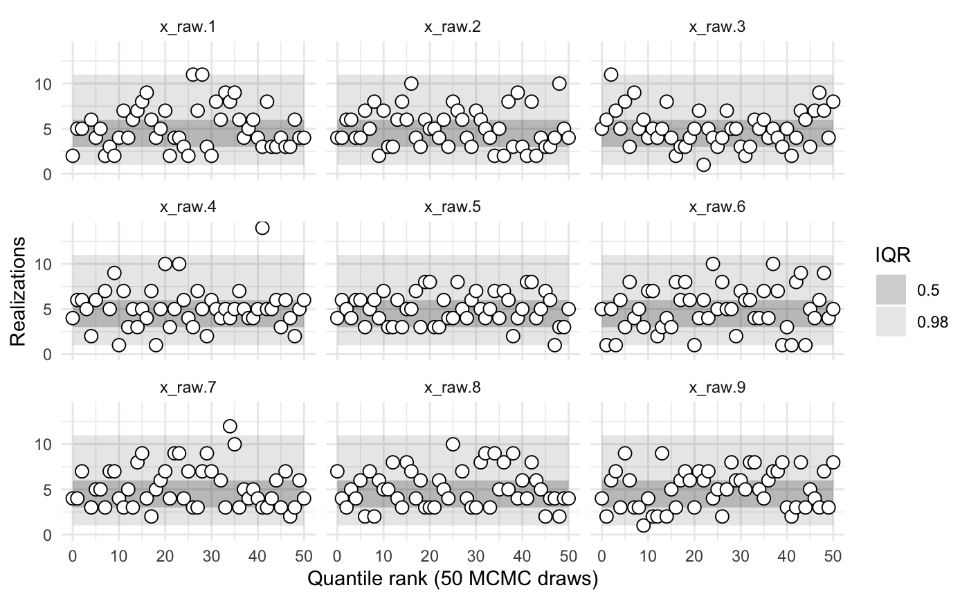
sbc2a$summary()
#> 
#> 
#>    iq expected.outside actual.outside
#>  0.50             0.50      0.4313725
#>  0.98             0.02      0.0000000

Rather than comparing simulated and sampled values of x_raw and y_raw, we might instead wish to compare x and y. In the code that creates the object sbc2b, note that the params() function returns a list with named values x and y. Hence the calibration is performed on those parameters.

sbc2b <- SBC$new(
  params = function(seed, data) {
    set.seed(seed + 10)
    y_raw <- rnorm(1, 0, 1)
    x_raw <- rnorm(9, 0, 1)
    y <- 3.0 * y_raw;
    x <- exp(y/2) * x_raw;
    list(x = x, y = y)
  }, 
  sampling = function(seed, data, params, modeled_data, iters) {
    sampling(funnel_reparameterized, data = data, seed = seed, chains = 1, iter = 2 * iters, warmup = iters)
  })

Perform the calibration.

sbc2b$calibrate(N = 256, L = 50)
sbc2b$plot()

sbc2b$plot('y')

sbc2b$plot('x')

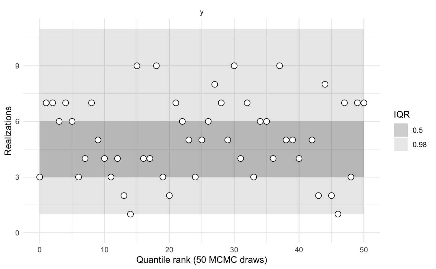
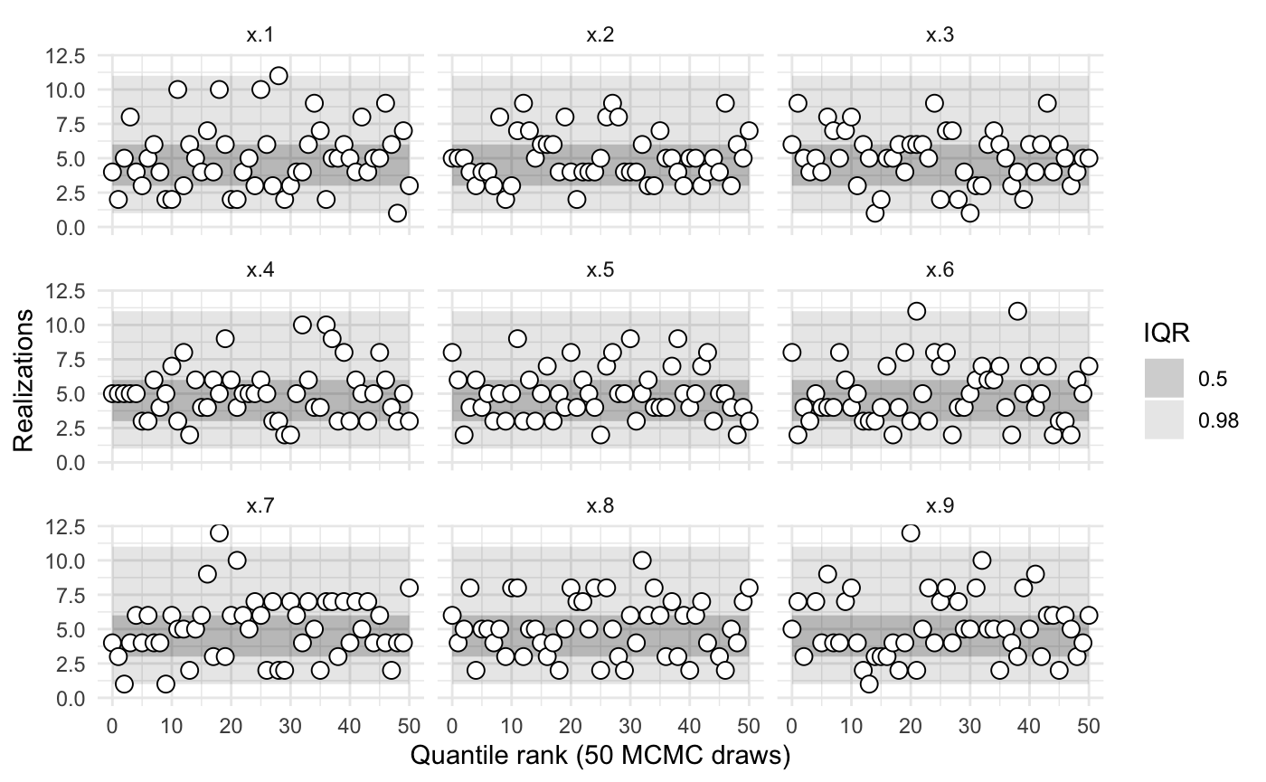
sbc2b$summary()
#> 
#> 
#>    iq expected.outside actual.outside
#>  0.50             0.50      0.3921569
#>  0.98             0.02      0.0000000

Both versions of the model are from https://mc-stan.org/docs/2_20/stan-users-guide/reparameterization-section.html ↩

Neal’s Funnel