Comparison to SBC implemented in rstan

library(sbcrs)
library(rstan)
#> Loading required package: StanHeaders
#> Loading required package: ggplot2
#> rstan (Version 2.19.2, GitRev: 2e1f913d3ca3)
#> For execution on a local, multicore CPU with excess RAM we recommend calling
#> options(mc.cores = parallel::detectCores()).
#> To avoid recompilation of unchanged Stan programs, we recommend calling
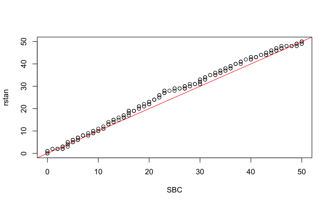
#> rstan_options(auto_write = TRUE)

We will compare the ranks calculated using the SBC package against those calculated by the rstan::sbc() function.

The stan code for this model is based on the help text for rstan::sbc. The following model is given as an example:

data {
  int<lower = 1> N;
  real<lower = 0> a;
  real<lower = 0> b;
}
transformed data { // these adhere to the conventions above
  real pi_ = beta_rng(a, b);
  int y = binomial_rng(N, pi_);
}
parameters {
  real<lower = 0, upper = 1> pi;
}
model {
  target += beta_lpdf(pi | a, b);
  target += binomial_lpmf(y | N, pi);
}
generated quantities { // these adhere to the conventions above
  int y_ = y;
  vector[1] pars_;
  int ranks_[1] = {pi > pi_};
  vector[N] log_lik;
  pars_[1] = pi_;
  for (n in 1:y) log_lik[n] = bernoulli_lpmf(1 | pi);
  for (n in (y + 1):N) log_lik[n] = bernoulli_lpmf(0 | pi);
}

Compile this Stan model:

sbc_rstan_model <- stan_model(file = system.file('stan', 'rstan_sbc_example.stan', package = 'sbcrs'))

Calibration involves generating data and parameters, and sampling from a Stan model many times. To speed up this process, take advantage of all of your machine’s cores.

doParallel::registerDoParallel(cores = parallel::detectCores())
options(mc.cores = parallel::detectCores())

Calibrate using rstan::sbc().

calibration_data <- list(N = 10, a = 2, b = 2)
rstan_sbc <- rstan::sbc(sbc_rstan_model, data = calibration_data, 256)
plot(rstan_sbc, binwidth = 1, thin = 50)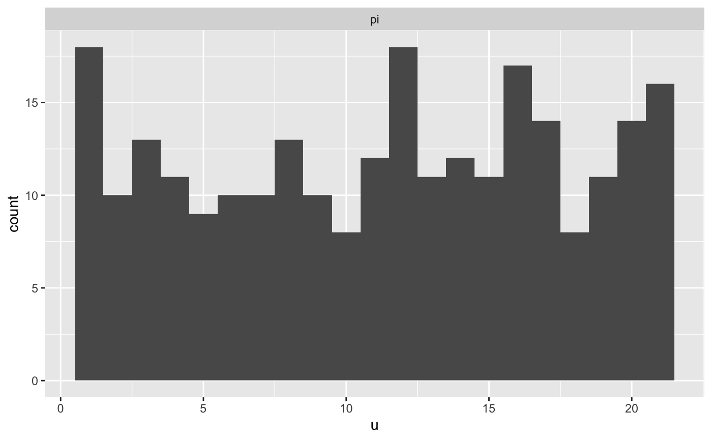

The Stan code used in the above example has been modified from the original. In the modified version, y is generated in the transformed data block of the Stan file. The original model would have looked like this:

data {
  int<lower = 1> N;
  real<lower = 0> a;
  real<lower = 0> b;
  int<lower = 0, upper = N> y;
}
parameters {
  real<lower = 0, upper = 1> pi;
}
model {
  target += beta_lpdf(pi | a, b);
  target += binomial_lpmf(y | N, pi);
}
generated quantities {
  real pi_ = beta_rng(a, b);

  vector[N] log_lik;
  for (n in 1:y) log_lik[n] = bernoulli_lpmf(1 | pi);
  for (n in (y + 1):N) log_lik[n] = bernoulli_lpmf(0 | pi);
}

Compile this Stan model:

sbc_original_model <- stan_model(file = system.file('stan', 'rstan_sbc_example_original.stan', package = 'sbcrs'))

Create an SBC object that corresponds with the original model.

sbc <- SBC$new(
  data = function(seed) {
    calibration_data
  },
  params = function(seed, data) {
    set.seed(seed + 1e6)
    list(pi = rbeta(1, data$a, data$b))
  },
  modeled_data = function(seed, data, params) {
    set.seed(seed + 2e6)
    list(y = rbinom(1, data$N, params$pi))
  },
  sampling = function(seed, data, params, modeled_data, iters) {
    sampling(sbc_original_model, data = c(data, modeled_data), seed = seed,
             chains = 1, iter = 2 * iters, warmup = iters)
  })

sbc$calibrate(256, 50)
sbc$plot()

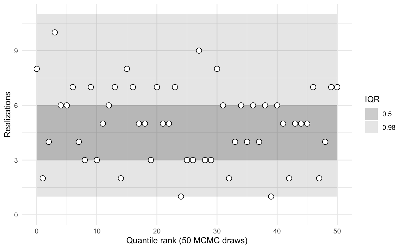
Assess whether the distributions of recovered ranks are similar

library(purrr)
x <- 
  map(sbc$calibrations, 'ranks') %>%
  flatten() %>%
  unlist() %>%
  unname()

y <- 
  rstan_sbc$ranks %>%
  map(~.x[seq(1, 1000, by = 20), ]) %>%
  map(~sum(.x)) %>%
  unlist()

qqplot(x, y, xlab = 'SBC', ylab = 'rstan')
abline(a = 0, b = 1, col = 'red')

wilcox.test(x, y)
#> 
#>  Wilcoxon rank sum test with continuity correction
#> 
#> data:  x and y
#> W = 30819, p-value = 0.2443
#> alternative hypothesis: true location shift is not equal to 0